Asymptotic Behavior

Control Engineering with Python

Symbols

🐍	Code	🔍	Worked Example
📈	Graph	🧩	Exercise
🏷️	Definition	💻	Numerical Method
💎	Theorem	🧮	Analytical Method
📝	Remark	🧠	Theory
ℹ️	Information	🗝️	Hint
⚠️	Warning	🔓	Solution

🐍 Imports

from numpy import *
from numpy.linalg import *
from scipy.linalg import *
from matplotlib.pyplot import *
from mpl_toolkits.mplot3d import *
from scipy.integrate import solve_ivp

🐍 Streamplot Helper

def Q(f, xs, ys):
    X, Y = meshgrid(xs, ys)
    v = vectorize
    fx = v(lambda x, y: f([x, y])[0])
    fy = v(lambda x, y: f([x, y])[1])
    return X, Y, fx(X, Y), fy(X, Y)

ℹ️ Assumption

From now on, we only deal with well-posed systems.

🏷️ Asymptotic

Asymptotic = Long-Term: when $t \to + \infty$

⚠️

Even simple dynamical systems may exhibit

complex asymptotic behaviors.

Lorenz System

$\begin{array}{lll} \dot{x} & = & σ (y - x) \\ \dot{y} & = & x (ρ - z) \\ \dot{z} & = & x y - β z \end{array}$

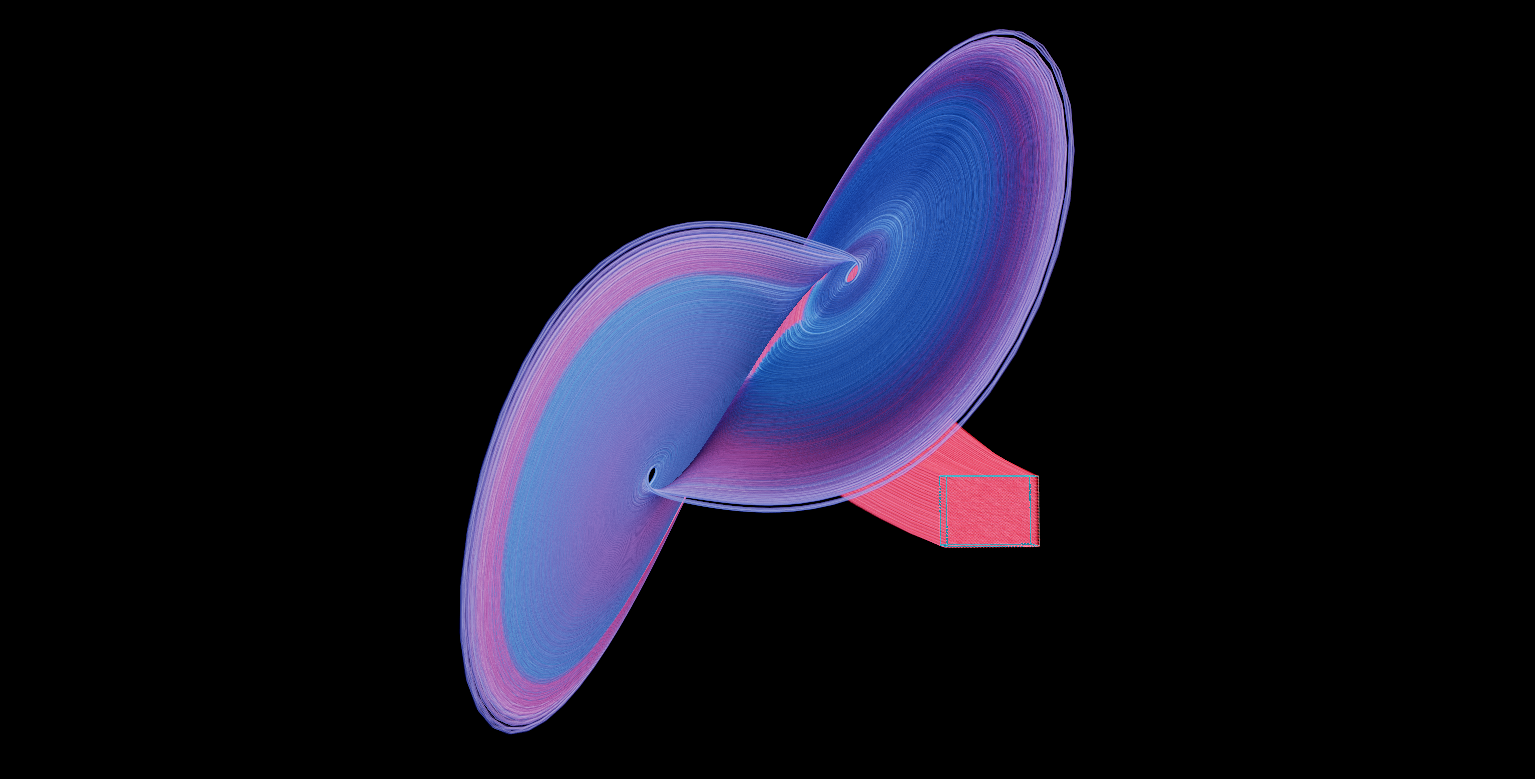
Visualized with Fibre

Hadley System

$\begin{array}{lll} \dot{x} & = & - y^{2} - z^{2} - a x + a f \\ \dot{y} & = & x y - b x z - y + g \\ \dot{z} & = & b x y + x z - z \end{array}$

Visualized with Fibre

🏷️ Equilibrium

An equilibrium of system $\dot{x} = f (x)$ is a state $x_{e}$ such that the maximal solution $x (t)$ such that $x (0) = x_{e}$

is global and,
is $x (t) = x_{e}$ for any $t > 0$ .

💎 Equilibrium

The state $x_{e}$ is an equilibrium of $\dot{x} = f (x)$

$⟺$

$f (x_{e}) = 0.$

Stability

About the long-term behavior of solutions.

“Stability” subtle concept,
“Asymptotic Stability” simpler (and stronger),
“Attractivity” simpler yet, (but often too weak).

Attractivity

Context: system $\dot{x} = f (x)$ with equilibrium $x_{e}$ .

🏷️ Global Attractivity

The equilibrium $x_{e}$ is globally attractive if for every $x_{0},$ the maximal solution $x (t)$ such that $x (0) = x_{0}$

is global and,
$x (t) \to x_{e}$ when $t \to + \infty$ .

🏷️ Local Attractivity

The equilibrium $x_{e}$ is locally attractive if for every $x_{0}$ close enough to $x_{e}$ , the maximal solution $x (t)$ such that $x (0) = x_{0}$

is global and,
$x (t) \to x_{e}$ when $t \to + \infty$ .

🔍 Global Attractivity

The system

$\begin{array}{cc} \dot{x} & = & - 2 x + y \\ \dot{y} & = & - 2 y + x \end{array}$

is well-posed,
has an equilibrium at $(0, 0)$ .

🐍 Vector field

def f(xy):
    x, y = xy
    dx = -2*x + y
    dy = -2*y + x
    return array([dx, dy])

📈 Stream plot

figure()
x = y = linspace(-5.0, 5.0, 1000)
streamplot(*Q(f, x, y), color="k")
plot([0], [0], "k.", ms=20.0)
axis("square")
axis("off")

🔍 Local Attractivity

The system

$\begin{array}{cc} \dot{x} & = & - 2 x + y^{3} \\ \dot{y} & = & - 2 y + x^{3} \end{array}$

is well-posed,
has an equilibrium at $(0, 0)$ .

🐍 Vector field

def f(xy):
    x, y = xy
    dx = -2*x + y**3
    dy = -2*y + x**3
    return array([dx, dy])

📈 Stream plot

figure()
x = y = linspace(-5.0, 5.0, 1000)
streamplot(*Q(f, x, y), color="k")
plot([0], [0], "k.", ms=10.0)
axis("square")
axis("off")

🔍 No Attractivity

The system

$\begin{array}{cr} \dot{x} & = & - 2 x + y \\ \dot{y} & = & 2 y - x \end{array}$

is well-posed,
has a (unique) equilibrium at $(0, 0)$ .

🐍 Vector field

def f(xy):
    x, y = xy
    dx = -2*x + y
    dy =  2*y - x
    return array([dx, dy])

📈 Stream plot

figure()
x = y = linspace(-5.0, 5.0, 1000)
streamplot(*Q(f, x, y), color="k")
plot([0], [0], "k.", ms=10.0)
axis("square")
axis("off")

🧩 Pendulum

The pendulum is governed by the equation

$m ℓ^{2} \ddot{θ} + b \dot{θ} + m g ℓ \sin θ = 0$

where $m > 0$ , $ℓ > 0$ , $g > 0$ and $b \geq 0$ .

1. 🧮

Compute the equilibria of this system.

2. 🧠

Can any of these equilibria be globally attractive?

3. 📈

Assume that $m = 1$ , $ℓ = 1$ , $g = 9.81$ and $b = 1$ .

Make a stream plot of the system.

4. 🔬

Determine which equilibria are locally attractive.

5. 📈 Frictionless Pendulum

Assume now that $b = 0$ .

Make a stream plot of the system.

6. 🧮 🧠

Prove that the equilibrium at $(0, 0)$ is not locally attractive.

🗝️ Hint. Study how the total mechanical energy $E$

$E (θ, \dot{θ}) := m ℓ^{2} {\dot{θ}}^{2} / 2 - m g ℓ \cos θ$

evolves in time.

🔓 Pendulum

1. 🔓

The 2nd-order differential equations of the pendulum are equivalent to the first order system

$| \begin{array}{rcl} \dot{θ} & = & ω \\ \dot{ω} & = & (- b / m ℓ^{2}) ω - (g / ℓ) \sin θ \end{array}$

Thus, the system state is $x = (θ, ω)$ and is governed by $\dot{x} = f (x)$ with

$f (θ, ω) = (ω, (- b / m ℓ^{2}) ω - (g / ℓ) \sin θ) .$

Hence, the state $(θ, ω)$ is a solution to $f (θ, ω) = 0$ if and only if $ω = 0$ and $\sin θ = 0$ . In other words, the equilibria of the system are characterized by $θ = k π$ for some $k \in Z$ and $ω (= \dot{θ}) = 0$ .

2. 🔓

Since there are several equilibria, none of them can be globally attractive.

Indeed let $x_{1}$ be a globally attractive equilibrium and assume that $x_{2}$ is any other equilibrium. By definition, the maximal solution $x (t)$ such that $x (0) = x_{2}$ is $x (t) = x_{2}$ for every $t \geq 0$ . On the other hand, since $x_{1}$ is globally attractive, it also satisfies $x (t) \to x_{1}$ when $t \to + \infty$ , hence there is a contradiction.

Thus, $x_{1}$ is the only possible equilibrium.

3. 🔓

m = l = b = 1; g=9.81

def f(theta_omega):
    theta, omega = theta_omega
    d_theta = omega
    d_omega = - b / (m * l * l) * omega
    d_omega -=  (g / l) * sin(theta)
    return (d_theta, d_omega)

figure()
theta = linspace(-2*pi*(1.2), 2*pi*(1.2), 1000)
d_theta = linspace(-5.0, 5.0, 1000)
streamplot(*Q(f, theta, d_theta), color="k")
plot([-2*pi, -pi, 0 ,pi, 2*pi], 5*[0.0], "k.")
xticks([-2*pi, -pi, 0 ,pi, 2*pi],
[r"$-2\pi$", r"$\pi$", r"$0$", r"$\pi$", r"$2\pi$"])
grid(True)

4. 🔓

From the streamplot, we see that the equilibria

$(θ, \dot{θ}) = (2 k π, 0), k \in Z$

are asymptotically stable, but that the equilibria

$(θ, \dot{θ}) = (2 (k + 1) π, 0), k \in Z$

are not (they are not locally attractive).

5. 🔓

b = 0
figure()
streamplot(*Q(f, theta, d_theta), color="k")
plot([-2*pi, -pi, 0 ,pi, 2*pi], 5*[0.0], "k.")
xticks([-2*pi, -pi, 0 ,pi, 2*pi],
[r"$-2\pi$", r"$\pi$", r"$0$", r"$\pi$", r"$2\pi$"])
grid(True)

6. 🔓

$\begin{aligned} \dot{E} & = \frac{d}{d t} (m ℓ^{2} {\dot{θ}}^{2} / 2 - m g ℓ \cos θ) \\ = m ℓ^{2} \ddot{θ} \dot{θ} + m g ℓ (\sin θ) \dot{θ} \\ = (m ℓ^{2} \ddot{θ} + m g ℓ \sin θ) \dot{θ} \\ = (- b \dot{θ}) \dot{θ} \\ = 0 \end{aligned}$

Therefore, $E (t)$ is constant.

On the other hand,

$min {E (θ, \dot{θ}) | (θ, \dot{θ}) \in R^{2}} = E (0, 0) = - m g l .$

Moreover, this minimum is locally strict. Precisely, for any $0 < | θ | < π$ , $E (0, 0) < E (θ, \dot{θ}) .$

If the origin was locally attractive, for any $θ (0)$ and $\dot{θ} (0)$ small enough, we would have $E (θ (t), \dot{θ} (t)) \to E (0, 0) when t \to + \infty$ (by continuity). But if $0 < | θ (0) | < π$ , we have

$E (θ (0), \dot{θ} (0)) > E (0, 0)$

and that would contradict that $E (t)$ is constant.

Hence the origin is not locally attractive.

💎 Attractivity (Low-level)

The equilibrium $x_{e}$ is globally attractive iff:

for any state $x_{0}$ and for any $ϵ > 0$ there is a $τ \geq 0$ ,
such that the maximal solution $x (t)$ such that $x (0) = x_{0}$ is global and,
satisfies:

$∥ x (t) - x_{e} ∥ \leq ϵ when t \geq τ .$

⚠️ Warning

Very close values of $x_{0}$ could theoretically lead to very different “speed of convergence” of $x (t)$ towards the equilibrium.
This is not contradictory with the well-posedness assumption: continuity w.r.t. the initial condition only works with finite time spans.

🔍 (Pathological) Example

$\begin{array}{lll} \dot{x} & = & x + x y - (x + y) \sqrt{x^{2} + y^{2}} \\ \dot{y} & = & y - x^{2} + (x - y) \sqrt{x^{2} + y^{2}} \end{array}$

Equivalently, in polar coordinates:

$\begin{array}{lll} \dot{r} & = & r (1 - r) \\ \dot{θ} & = & r (1 - \cos θ) \end{array}$

🐍 Vector Field

def f(xy):
    x, y = xy
    r = sqrt(x*x + y*y)
    dx = x + x * y - (x + y) * r
    dy = y - x * x + (x - y) * r
    return array([dx, dy])

📈 Stream Plot

figure()
x = y = linspace(-2.0, 2.0, 1000)
streamplot(*Q(f, x, y), color="k")
plot([1], [0], "k.", ms=20.0)
axis("square")
axis("off")

Asymptotic Stability

Asymptotic stability is a stronger version of attractivity which is by definition robust with respect to the choice of the initial state.

🏷️ Global Asympt. Stability

The equilibrium $x_{e}$ is globally asympt. stable iff:

for any state $x_{0}$ and for any $ϵ > 0$ there is a $τ \geq 0$ ,
and there is a $r > 0$ such that if $∥ x_{0}^{'} - x_{0} ∥ \leq r$ ,
such that the maximal solution $x (t)$ such that $x (0) = x_{0}^{'}$ is global and,
satisfies:

$∥ x (t) - x_{e} ∥ \leq ϵ when t \geq τ .$

Set of Initial Conditions

Let $f : R^{n} \to R^{n}$ and $X_{0} \subset R^{n}$ .

Let $X (t)$ be the image of $X_{0}$ by the flow at time $t$ :

$X (t) := {x (t) | \dot{x} = f (x), x (0) = x_{0}, x_{0} \in X_{0}} .$

💎 Global Asympt. Stability

An equilibrium $x_{e}$ is globally asympt. stable iff

for every bounded set $X_{0}$ and any $x_{0} \in X_{0}$ the associated maximal solution $x (t)$ is global and,
$X (t) \to {x_{e}}$ when $t \to + \infty$ .

🏷️ Limits of Sets

$X (t) \to {x_{e}}$

to be interpreted as

$sup_{x (t) \in X (t)} ∥ x (t) - x_{e} ∥ \to 0.$

🏷️ Hausdorff Distance

$sup_{x (t) \in X (t)} ∥ x (t) - x_{e} ∥ = d_{H} (X (t), {x_{e}})$

where $d_{H}$ is the Hausdorff distance between sets:

$d_{H} (A, B) := max {sup_{a \in A} d (a, B), sup_{b \in B} d (A, b)} .$

🏷️ Local Asymptotic Stability

The equilibrium $x_{e}$ is locally asympt. stable iff:

there is a $r > 0$ such that for any $ϵ > 0$ ,
there is a $τ \geq 0$ such that,
if $∥ x_{0} - x_{e} ∥ \leq r$ , the maximal solution $x (t)$ such that $x (0) = x_{0}$ is global and satisfies:

$∥ x (t) - x_{e} ∥ \leq ϵ when t \geq τ .$

💎 Local Asympt. Stability

An equilibrium $x_{e}$ is locally asympt. stable iff:

There is a $r > 0$ such that for every set $X_{0}$ such that

$X_{0} \subset {x | ∥ x - x_{e} ∥ \leq r},$

and for any $x_{0} \in X_{0}$ , the associated maximal solution $x (t)$ is global and

$X (t) \to {x_{e}} when t \to + \infty .$

🏷️ Stability

An equilibrium $x_{e}$ is stable iff:

for any $r > 0$ ,
there is a $ρ \leq r$ such that if $| x (0) - x_{e} | \leq ρ$ , then
the solution $x (t)$ is global,
for any $t \geq 0$ , $| x (t) - x_{e} | \leq r$ .

🧩 Vinograd System

Consider the system:

$\begin{array}{rcl} \dot{x} & = & (x^{2} (y - x) + y^{5}) / (x^{2} + y^{2} (1 + (x^{2} + y^{2})^{2})) \\ \dot{y} & = & y^{2} (y - 2 x) / (x^{2} + y^{2} (1 + (x^{2} + y^{2})^{2})) \end{array}$

🐍 Vector field

def f(xy):
    x, y = xy
    q = x**2 + y**2 * (1 + (x**2 + y**2)**2)
    dx = (x**2 * (y - x) + y**5) / q
    dy = y**2 * (y - 2*x) / q
    return array([dx, dy])

📈 Stream plot

figure()
x = y = linspace(-1.0, 1.0, 1000)
streamplot(*Q(f, x, y), color="k")
xticks([-1, 0, 1])
plot([0], [0], "k.", ms=10.0)
axis("square")
axis("off")

1. 🧮

Show that the origin $(0, 0)$ is the unique equilibrium.

2. 📈🔬

Does this equilibrium seem to be attractive (graphically) ?

3. 🧠

Show that for any equilibrium of a well-posed system:

💎 (locally) asymptotically stable $\Rightarrow$ stable

4. 🧪📈

Does the origin seem to be stable (experimentally ?)

Conclude accordingly.

🔓 Vinograd System

1. 🔓

$(x, y)$ is an equilibrium of the Vinograd system iff

$\begin{array}{rcl} (x^{2} (y - x) + y^{5}) / (x^{2} + y^{2} (1 + (x^{2} + y^{2})^{2})) & = & 0 \\ y^{2} (y - 2 x) / (x^{2} + y^{2} (1 + (x^{2} + y^{2})^{2})) & = & 0 \end{array}$

or equivalently

$y^{2} (y - 2 x) = 0 and x^{2} (y - x) + y^{5} = 0.$

If we assume that $y = 0$ , then:

$y^{2} (y - 2 x) = 0$ is satisfied and
$x^{2} (y - x) + y^{5} = 0 \Leftrightarrow - x^{3} = 0 \Leftrightarrow x = 0.$

Under this assumption, $(0, 0)$ is the only equilibrium.

Otherwise (if $y \neq 0$ ),

$y^{2} (y - 2 x) = 0$ yields $y = 2 x$ ,
The substitution of $y$ by $2 x$ in $x^{2} (y - x) + y^{5} = 0$ yields $x^{3} (1 + 32 x^{2}) = 0$ and therefore $x = 0$ .
$y^{2} (y - 2 x) = 0$ becomes $y^{3} = 0$ and thus $y = 0$ .

The initial assumption cannot hold.

Conclusion:

The Vinograd system has a single equilibrium: $(0, 0)$ .

2. 🔓

Yes, the origin seems to be (globally) attractive.

As far as we can tell, the streamplot displays trajectories that ultimately all converge towards the origin.

3. 🔓

Let’s assume that $x_{e}$ is a (locally) asymptotically stable of a well-posed system.

Let $r > 0$ such that this property is satisfied and let

$B := {x \in R^{n} | ∥ x - x_{e} ∥ \leq r} \subset dom f .$

The set $x (t, B)$ is defined for any $t \geq 0$ and since $B$ is a neighbourhood of $x_{e}$ , there is $τ \geq 0$ such that for any $t \geq τ$ , the image of $B$ by $x (t, \cdot)$ is included in $B$ .

$t \geq τ \Rightarrow x (t, B) \subset B .$

Additionally, the system is well-posed.

Hence there is a $r^{'} > 0$ such that for any $x_{0}$ in the closed ball $B^{'}$ of radius $r^{'}$ centered at $x_{e}$ and any $t \in [0, τ]$ , we have

$∥ x (x_{0}, t) - x (x_{e}, t) ∥ \leq r .$

Since $x_{e}$ is an equilibrium, $x (t, x_{e}) = x_{e}$ , thus $∥ x (x_{0}, t) - x_{e} ∥ \leq r .$ Equivalently,

$0 \leq t \leq τ \Rightarrow x (t, B^{'}) \subset B .$

Note that since $x (0, B^{'}) = B^{'}$ , this inclusion yields $B^{'} \subset B$ . Thus, for any $t \geq 0$ , either $t \in [0, τ]$ and $x (t, B^{'}) \subset B$ or $t \geq τ$ and since $B^{'} \subset B$ ,

$x (t, B^{'}) \subset x (t, B) \subset B .$

Conclusion: we have established that there is a $r > 0$ such that $B \subset dom f$ and a $r^{'} > 0$ such that $r^{'} \leq r$ and

$t \geq 0 \Rightarrow x (t, B^{'}) \subset B .$

In other words, the system is stable! 🎉

4. 🔓

No! We can pick initial states $(0, ε)$ , with $ε > 0$ which are just above the origin and still the distance of their trajectory to the origin will exceed $1.0$ at some point:

def fun(t, xy):
    return f(xy)
eps = 1e-10; xy0 = (0, eps)
sol = solve_ivp(
  fun=fun,
  y0=xy0,
  t_span=(0.0, 100.0),
  dense_output=True)["sol"]

t = linspace(0.0, 100.0, 10000)
xt, yt = sol(t)
figure()
x = y = linspace(-1.0, 1.0, 1000)
streamplot(*Q(f, x, y), color="#ced4da")
xticks([-1, 0, 1])
plot([0], [0], "k.", ms=10.0)
plot(xt, yt, color="C0")