Functions
Function definition, arguments, generators, closures, and decorators

Sébastien Boisgérault
Associate Professor, ITN Mines Paris – PSL
Functions
Generalities
Functions are defined using the keyword def, followed by the name of the function,
followed by the list of their parameters in parentheses.
The return value of a function is preceded by the keyword return.
def fibonacci(n):
    "Return a list of n Fibonacci numbers."
    result = []
    a, b = (0, 1)
    while len(result) < n:
        result.append(a)
        a, b = b, a+b
    return result
To call the function fibonacci passing as argument the argument 10 and retrieve the result:
>>> numbers = fibonacci(10)
>>> numbers
[0, 1, 1, 2, 3, 5, 8, 13, 21, 34]
The parameters of a function can be accompanied by a default value.
We can thus add a second parameter start to the function fibonacci with default value (0, 1).
def fibonacci(n, start=(0, 1)):
    "Return a list of n Fibonacci numbers."
    result = []
    a, b = start
    while len(result) < n:
        result.append(a)
        a, b = b, a+b
    return result
If we do not specify the value of the parameter at invocation, its default value is used.
In this case, if we do not give a second argument to the function fibonacci,
it behaves like the first version:
>>> numbers = fibonacci(10)
>>> numbers
[0, 1, 1, 2, 3, 5, 8, 13, 21, 34]
However, if we provide a second argument, the default value is not used.
>>> numbers = fibonacci(10, (21, 34))
>>> numbers
[21, 34, 55, 89, 144, 233, 377, 610, 987, 1597]
Note that arguments can generally be positional — the parameter to which the argument
is assigned depends on the position of the argument in the list of arguments passed to the function —
or keyword (named), in which case the argument is assigned to the parameter of the same name.
Keyword arguments are often useful to make the role of the argument clearer.
Thus, the second argument of fibonacci, named start, is a pair of integers
that provides the two initial values of the Fibonacci sequence. The role of the code is
probably more obvious if we use a keyword argument:
>>> numbers = fibonacci(10, start=(21, 34))
>>> numbers
[21, 34, 55, 89, 144, 233, 377, 610, 987, 1597]
Note that the use of keyword arguments also makes it possible to ignore
the order in which the parameters of the function are specified:
>>> numbers = fibonacci(start=(21, 34), n=10)
>>> numbers
[21, 34, 55, 89, 144, 233, 377, 610, 987, 1597]
Arguments: * and **
It is possible to store values in a tuple1, then use them as positional arguments
in a call to a function. For example:
>>> args = (10, (21, 34))
>>> fibonacci(*args)
[21, 34, 55, 89, 144, 233, 377, 610, 987, 1597]
A similar mechanism exists with dictionaries and keyword arguments:
>>> kwargs = {"n": 10, "start": (21, 34)}
>>> fibonacci(**kwargs)
[21, 34, 55, 89, 144, 233, 377, 610, 987, 1597]
It is possible to hybridize the two approaches:
>>> args = (10,)
>>> kwargs = {"start": (21, 34)}
>>> fibonacci(*args, **kwargs)
[21, 34, 55, 89, 144, 233, 377, 610, 987, 1597]
There is also a form of symmetry in this mechanism, which can be
used to define a function that accepts an arbitrary number of
positional and/or keyword arguments. For example, with:
def f(*args, **kwargs):
    print(f"args = {args!r}")
    print(f"kwargs = {kwargs!r}")
We get:
>>> f(1, "Hello!")
args = (1, 'Hello!')
kwargs = {}
>>> f(fast=True, verbose=False)
args = ()
kwargs = {'fast': True, 'verbose': False}
Static Typing
Python is a dynamically typed language; the same variable can denote
an integer at one moment and a string at another. However,
it is possible — but optional — to statically attach a
type annotation
to a variable.
For example, if you want to declare that the function fibonacci takes
an integer and a pair of integers as arguments and returns a list of integers,
you can define it as follows:
def fibonacci(
    n: int,
    start: tuple[int, int] = (0, 1)
) -> list[int]:
    "Return a list of n Fibonacci numbers."
    result : list[int] = []
    a, b = start
    while len(result) < n:
        result.append(a)
        a, b = b, a+b
    return result
This information can be used during development to detect any structural inconsistencies
in your code. Thus, if you complete the code above with:
fibonacci("Hello!", True)
The use of mypy will provide:
$ mypy fib.py
fibonacci.py:13: error: Argument 1 to "fibonacci" has incompatible type "str"; expected "int"
fibonacci.py:13: error: Argument 2 to "fibonacci" has incompatible type "bool"; expected "Tuple[int, int]"
Found 2 errors in 1 file (checked 1 source file)
Namespaces
The scope of a variable in a program determines the way it is associated with a value.
At the top level (of a file, a module, the Python interpreter, etc.),
variables are global. The link between the variable name and
the value it designates is described by the globals() dictionary:
this is the namespace associated with global variables.
>>> import math
>>> message = "Hello world"
>>> def answer():
...    return 42
...
>>> globs = globals()
>>> globs["math"] is math
True
>>> globs["message"] is message
True
>>> globs["answer"] is answer
True
Within functions, there are generally local variables to the function.
This is notably the case of the function parameters, and — in the absence of
a contrary statement — variables assigned within it. In the body of this function,
the associated namespace can be obtained by calling locals().
>>> x = 1
>>> def f(y):
...     z = 3
...     locs = locals()
...     print("x" in locs)
...     print("y" in locs)
...     print("z" in locs)
...
>>> f(2)
False
True
True
It is therefore possible for a local variable to shadow a global variable:
>>> a = 1
>>> def f():
...     a = 2  # assigned => local
...     print(a)
...
>>> a
1
>>> f()
2
>>> a  # in the global scope => the value remains unchanged
1
In the absence of such an assignment, within a function, global variables remain accessible,
but only for reading:
>>> a = 1
>>> def f():
...     print(a)
...
>>> f()
1
If we want to assign a new value to a global variable within the body of a function,
it is necessary to declare the variable as global:
>>> a = 1
>>> def f():
...     global a
...     a = 2
...
>>> print(a)
1
>>> f()
>>> print(a)
2
There is also a built-in scope and in the case of nested functions,
the concept of outer scope; see for example
the description of the LEGB rule.
Callables
An object that behaves like a function, that is, can be called (invoked) with the
same syntax as functions, is called a callable.
Thus, the integer 0 is not callable:
>>> zero = 0
>>> zero()
Traceback (most recent call last):
  File "<stdin>", line 1, in <module>
TypeError: 'int' object is not callable
But the function without argument that returns 0 is callable:
>>> def zero_fun():
...     return 0
...
>>> zero_fun()
0
Which is not a surprise since it is a function!
>>> type(zero_fun)
<class 'function'>
>>> import types
>>> isinstance(zero_fun, types.FunctionType)
True
The callability of Python objects can be tested with the function callable:
>>> callable(zero)
False
>>> callable(zero_fun)
True
Note that this test tells whether an object is callable, but not whether it can be
invoked without arguments (or how many arguments are needed, of what type, etc.). Thus:
>>> callable(hash)
True
But:
>>> hash()
Traceback (most recent call last):
  File "<stdin>", line 1, in <module>
TypeError: hash() takes exactly one argument (0 given)
However:
>>> hash(2**100)
549755813888
To learn more about the expected arguments, refer to the documentation of the
object in question.
Types
An object like int is also callable:
>>> callable(int)
True
Which can be quickly confirmed experimentally:
>>> int()
0
>>> int(0.0)
0
>>> int("0")
0
Yet it is not a function, but a type:
>>> type(int)
<class 'type'>
>>> type(int) is type  # 🤯
True
>>> isinstance(int, types.FunctionType)
False
Recall that types (or classes) are intended, when called, to create
instances of the type considered:
>>> isinstance(int(), int)
True
>>> isinstance(int(0.0), int)
True
>>> isinstance(int("0"), int)
True
The classes you define are also callable:
class Transmogrifier:
    pass
>>> callable(Transmogrifier)
True
>>> transmogrifier = Transmogrifier()
>>> isinstance(transmogrifier, Transmogrifier)
True
Methods
A transmogrifier
can transform its user into whatever it wants (by default, a tiger 🐯;
but we didn’t specify the size of the tiger! 😉).

Calvin (on the right) transformed into a tiger
class Transmogrifier:
    def __init__(self, turn_into="tiger"):
        self.turn_into = turn_into
    def activate(self, user):
        return self.turn_into
>>> transmogrifier = Transmogrifier()
>>> transmogrifier.activate("calvin")
'tiger'
The operation transmogrifier.activate("calvin") is not “atomic”: it first obtains
the attribute activate from the object transmogrifier, then invokes it
with the argument "calvin".
>>> transmogrify = transmogrifier.activate
>>> callable(transmogrify)
True
>>> transmogrify("calvin")
'tiger'
This is possible because activate is a method (bound to the instance
transmogrifier of Transmogrifier) and is therefore callable.
>>> transmogrify
<bound method Transmogrifier.activate ...>
>>> type(transmogrify)
<class 'method'>
>>> import types
>>> type(transmogrify) is types.MethodType
True
Instances
Note that at this stage Transmogrifier is callable and the method activate
of transmogrifiers is also callable. But the transmogrifiers themselves are not:
>>> callable(transmogrifier)
False
If we think it is preferable, we can make them callable. It seems quite reasonable
to make invoking a transmogrifier activate it:
class Transmogrifier:
    def __init__(self, turn_into="tiger"):
        self.turn_into = turn_into
    def activate(self, user):
        return self.turn_into
    def __call__(self, user):
        return self.activate(user)
>>> transmogrifier = Transmogrifier()
>>> callable(transmogrifier)
True
We can then simplify the usage of the transmogrifier as follows:
>>> transmogrifier("calvin")
'tiger'
Generator Functions
A function is generator if its definition uses the keyword yield.
-
Calling a generator function does not execute its code immediately,
but returns an iterator as return value.
-
Accessing the first element of this iterator executes the function until
it reaches the first yield; the function then returns the value provided
to yield, then pauses its execution.
-
Accessing the second element of this iterator resumes execution
from that point, until it reaches the second yield, etc.
Thus, with
def one_two_three():
    yield 1
    yield 2
    yield 3
We get:
>>> for i in one_two_three():
...     print(i)
...
1
2
3
And:
>>> list(one_two_three())
[1, 2, 3]
def count(start=0, step=1):
    """
    Generate the sequence start, start + step, start + 2*step, ...
    """
    value = start
    while True:
        yield value
        value += step
Usage:
>>> odd_numbers = count(start=1, step=2)
>>> for number in odd_numbers:
...     if number >= 20:
...         break
...     else:
...         print(number)
...
1
3
5
7
9
11
13
15
17
19
def cycle(iterable):
    """
    Yield all items from an iterable, then repeat this sequence indefinitely.
    """
    items = list(iterable)
    while items:
        for item in items:
            yield item
Usage:
>>> for i, item in enumerate(cycle("ABCD")):
...     if i >= 12:
...         break
...     else:
...         print(item)
...
A
B
C
D
A
B
C
D
A
B
C
D
def repeat(object, n=None):
    """
    Yield object an object n times (or indefinitely if n is None).
    """
    if n is None:
        while True:
            yield object
    else:
        for i in range(n):
            yield object
Usage:
>>> list(repeat(10, 3))
[10, 10, 10]
Exercises
-
Implement your own version of the standard functions range, enumerate
and zip using generator functions.
-
Review the definition of the function fibonacci to make it a generator
function that returns Fibonacci numbers as an iterator rather than a list.
Make sure that when argument n is not provided, the iterator traverses
the entire sequence.
Functional Programming
One of the features of functional programming2, a style of programming that
Python supports (in part), is to allow manipulation of functions as
objects like others, which can be assigned to variables, stored in containers,
passed as arguments to other functions, etc. A function that accepts
functions as arguments and/or returns functions is a higher-order function.
Mathematical libraries often make good use of these higher-order functions.
Thus, the Autograd automatic differentiation library defines a higher-order function
grad that associates with a real-valued function its derivative.
Its documentation gives the following example of usage:
>>> import autograd.numpy as np
>>> from autograd import grad
>>> def tanh(x):
...     y = np.exp(-2.0 * x)
...     return (1.0 - y) / (1.0 + y)
...
>>> d_tanh = grad(tanh)  # d_tanh is the derivative of tanh
>>> d_tanh(1.0)          # we evaluate it at x = 1.0
0.419974341614026
Another important use of higher-order functions is the exploitation of
callback functions, notably in graphical interfaces.
For example, let’s look at how the graphical application given as an example
in the Tk library tutorial is programmed:
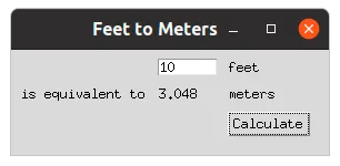
The graphical interface is partly defined by the code:
from tkinter import *
from tkinter import ttk

root = Tk()
root.title("Feet to Meters")

mainframe = ttk.Frame(root, padding="3 3 12 12")
mainframe.grid(column=0, row=0, sticky=(N, W, E, S))
root.columnconfigure(0, weight=1)
root.rowconfigure(0, weight=1)

feet = StringVar()
feet_entry = ttk.Entry(mainframe, width=7, textvariable=feet)
feet_entry.grid(column=2, row=1, sticky=(W, E))

meters = StringVar()
ttk.Label(mainframe, textvariable=meters).grid(column=2, row=2, sticky=(W, E))
Let’s just note at this stage that feet is the text field where we enter
the length in feet and meters is the text field that should display
the equivalent length in meters when we click the button.
For the application to behave as desired, we define a function calculate
that each time it is invoked, reads the length in feet and writes the length
in meters:
def calculate(*args):
    try:
        value = float(feet.get())
        meters_value = int(0.3048 * value * 1e4 + 0.5) / 1e4
        meters.set(meters_value)
    except ValueError:
        pass
Then we create a button that calls back this function each time it is pressed:
ttk.Button(
    mainframe,
    text="Calculate",
    command=calculate
).grid(column=3, row=3, sticky=W)
A few more labels in the graphical interface, a little bit of positioning,
and we are ready to launch the execution loop!
ttk.Label(mainframe, text="feet").grid(column=3, row=1, sticky=W)
ttk.Label(mainframe, text="is equivalent to").grid(column=1, row=2, sticky=E)
ttk.Label(mainframe, text="meters").grid(column=3, row=2, sticky=W)

for child in mainframe.winfo_children():
    child.grid_configure(padx=5, pady=5)

feet_entry.focus()

root.mainloop()
Lambda
Lambda functions in Python are a construct that does not increase
the expressiveness of the language — you can’t do anything with lambda
functions that you couldn’t already do with regular functions —
but in some cases allows for more concise code.
Thus, to numerically find the zero of the function $x \mapsto x^2 - 2$
between 0 and 2 with scipy, after importing a root-finding function:
from scipy.optimize import root_scalar as find_root
We can define the function of interest, which requires naming it
(for example f):
def f(x):
    return x*x - 2
Then call scipy’s zero-finding routine:
>>> find_root(f, bracket=[0, 2])
      converged: True
           flag: 'converged'
function_calls: 9
    iterations: 8
         root: 1.4142135623731364
But we can also skip the preliminary definition and naming step,
and perform this operation on the fly, in the call to find_root,
using a lambda function:
>>> find_root(lambda x: x*x-2, bracket=[0, 2])
      converged: True
           flag: 'converged'
function_calls: 9
    iterations: 8
         root: 1.4142135623731364
The keyword lambda refers to the traditional notation of
$\lambda$-calculus;
there, the function $x \mapsto x^2+1$ would be denoted
$(\lambda x.x^2+1)$.
Closures
As Wikipedia says:
In a programming language, a closure or clôture is a function
accompanied by its lexical environment.
The lexical environment of a function is the set of non-local variables
it has captured, either by value (i.e., by copying the values of the variables),
or by reference (i.e., by copying the memory addresses of the variables).
A closure is therefore created, among other things, when a function is defined
in the body of another function and uses parameters or local variables
of the latter.
Source: Closure (wikipedia)
Let’s try to give a concrete example illustrating this definition.
Expression Evaluator
The built-in function eval allows calculating the value of expressions
represented by strings. Thus:
>>> x = 1
>>> y = 2
>>> eval("x + y")
3
It is also possible to ignore the global namespace and explicitly specify
the namespace that the evaluator should use:
>>> namespace = {"x": 3, "y": 4}
>>> eval("x + y", namespace)
7
We would like to have a higher-order function — let’s call it fun —
that associates with an expression, like "x+y", a function that will accept
the necessary keyword arguments to evaluate the expression — here x and y —
and return the associated value of the expression.
With function closures, nothing could be simpler:
def fun(expression):
    def f(**kwargs):
       return eval(expression, kwargs)
    return f
Note that eval(expression, kwargs) uses the variable kwargs which is local to f
(because passed as parameter). But it also uses expression which is a local variable of fun;
it belongs to the lexical environment of f, which is therefore a closure.
Here’s how to use our function fun:
>>> add_xy = fun("x + y")
>>> add_xy(x=4, y=5)
9
--------------------------------------------------------------------------------

The non-local variables of a closure are accessible for reading by default.
To modify them, it is first necessary to explicitly declare them as non-local to the closure.
(The situation is therefore similar to that of global variables used in functions.)

For example, the function `make_get_set` generates two closures that access
the same variable `x` (which is local to `make_get_set`): `get` allows reading
the value of `x` and therefore does not need to declare it as non-local;
but `set` must be able to change the value of this variable and therefore declares it
as non-local:

```python
def make_get_set(x):
     def get():
         return x
     def set(value):
         nonlocal x
         x = value
     return get, set
Example usage of these functions:
>>> get, set = make_get_set(1)
>>> get()
1
>>> set(5)
>>> get()
5
--------------------------------------------------------------------------------

It is good to know that non-local variables are captured by reference in Python,
and not by value, which can in some cases make your life
... interesting! 😂

For example, the programmer who wrote:

```python
def make_actions():
    actions = []
    for i in range(3):
        def printer():
            print(i)
        actions.append(printer)
    return actions
Probably expects to generate a list of 3 actions that will display
0, 1 and 2 respectively when they are called.
But since i used by the function printer is captured by reference,
its effective value is determined only at the time of the call print(i). But at that time,
the for loop has already been executed, so i equals 2. Consequently, we actually get:
>>> for action in make_actions():
...     action()
...
2
2
2
The classic “hack” to solve this problem is to use the fact that the default
arguments of a function are evaluated at its definition.
Therefore, if we define:
def make_actions():
    actions = []
    for i in range(3):
        def printer(i=i):
            print(i)
        actions.append(printer)
    return actions
We get as desired:
>>> for action in make_actions():
...     action()
...
0
1
2
Decorators
Decorators are a syntactic sugar using the symbol @ that facilitates the
implementation of a fairly common pattern that we will illustrate with an example.
Imagine that we have developed a function plus_one
def plus_one(x):
    return x + 1
But in testing it in a program, we find its behavior mysterious.
To understand what is happening, we modify its definition to display
its arguments and the values it returns each time it is called.
def plus_one(x):
    print("input:", x)
    y = x + 1
    print("output:", y)
    return y
With the firm intention of removing this additional code once the mystery is solved.
However, this process is not very satisfactory. Rather than modifying
the code of plus_one, we can develop a function debug that takes the function
plus_one as an argument and returns a new function that works like plus_one
except that it displays the arguments and output value:
def debug(f):
    def f_debug(x):
        print("input:", x)
        y = f(x)
        print("output:", y)
        return y
    return f_debug
To test the code in a real situation, we just need to replace the classic function
plus_one with this new function
plus_one = debug(plus_one)
Then erase only this additional line once the mystery is solved.
It turns out that the code
def plus_one(x):
    return x + 1

plus_one = debug(plus_one)
Is equivalent to the following construction using the decorator @debug:
@debug
def plus_one(x):
    return x + 1
You may find this second notation more pleasant and readable!
Example
The higher-order function count below can be used as a decorator to record the number of times
a function has been invoked (the number of calls to the function is stored in the count attribute
of the function):
def count(f):
    def counted_f(x):
        counted_f.count += 1
        return f(x)
    counted_f.count = 0
    return counted_f
For example, if we want to locate the positive root of the function
$x \mapsto x^2 - 2$, which is $\sqrt2$, we can define it by decorating
it with @count:
@count
def f(x):
    return x*x - 2
Then proceed by successive iterations to produce an estimate of $\sqrt2$:
>>> f(0)
-2
>>> f(1)
-1
>>> f(2)
2
>>> f(1.5)
0.25
>>> f(1.4)
-0.04000000000000026
>>> f(1.45)
0.10250000000000004
>>> f(1.43)
0.04489999999999972
>>> f(1.42)
0.01639999999999997
>>> f(1.41)
-0.011900000000000244
And note afterward how many calls to the function f were necessary:
>>> f.count
9